TCLIB Suite
Software library & stand-alone tools for the optimization of telecentric setups
Key advantages
- State-of-the-art algorithms for distortion calibration.
- Ensure the best focus and alignment with fast and intuitive stand-alone tools.
- Maximize the system performance to achieve the best measurment results.
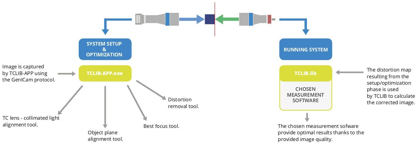
TCLIB Suite is a C++ based computer vision software designed to optimize the optical performances of a telecentric setup, typically used for measurement purposes. With the use of both a .dll library and dedicated stand-alone tools, TCLIB makes it easy to take care of all aspects of a typical telecentric setup (focusing, alignments, distortion calibration) which, if not properly addressed, can affect negatively the results of measurements.
TCLIB Suite helps improving the quality of the system, providing the best possible images for your chosen metrology software to get the best achievable measurement results. In fact, any edge detection, pattern matching and calibration software will be more accurate and reliable if based on well aligned, homogeneously backlit, undistorted images.
TCLIB APP is a full GenTL compliant software. Any GenTL compliant camera device can be used with this software. Camera manufacturer drivers need anyway to be installed in order for the program to operate correctly.
TCLIB Suite includes:
- Dedicated tools to take care of the basics of a measurement system setup: alignment of telecentric lens and collimated light, alignment of the object plane, best focus (TCLIB-APP)
- A set of algorithms (C++ library) to calculate the distortion map of a system and correct in live mode every new image acquired by the system (TCLIB), plus all the functions developed in the TCLIB-APP.
The stand-alone tools and the distortion calibration functions are used offline, when the initial optimization and calibration of the machine is needed. The distortion correction, on the other hand, is based on fast and reliable algorithms which allow the system to stream adjusted images in live mode.
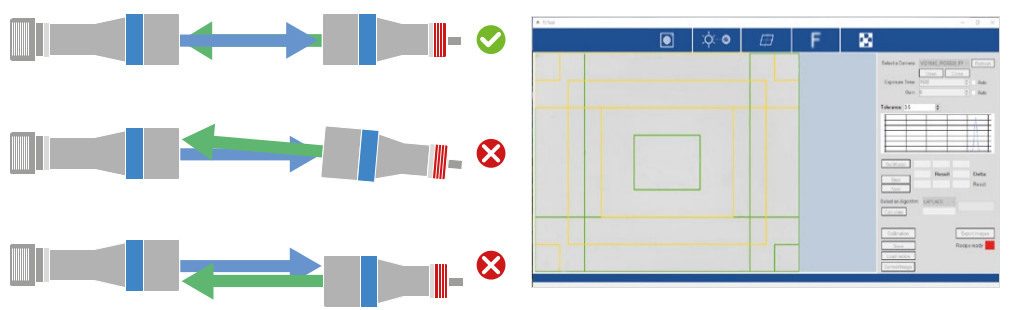
Aligning of lens and collimated light source
This tool assists the operator in getting the most homogeneous illumination possible.
Getting the best homogeneity of the illumination is the first fundamental step for a good measurement system, since this spec affecs thereliability of any set of edge detection algorithms.
The tool works in live mode, giving a visual feedback on the alignment. The FOV is divided in ROIs, each one having a color feedback regardingthe alignment:
- RED: not homogeneous
- YELLOW: discrete homogeneous
- GREEN: good homogeneous
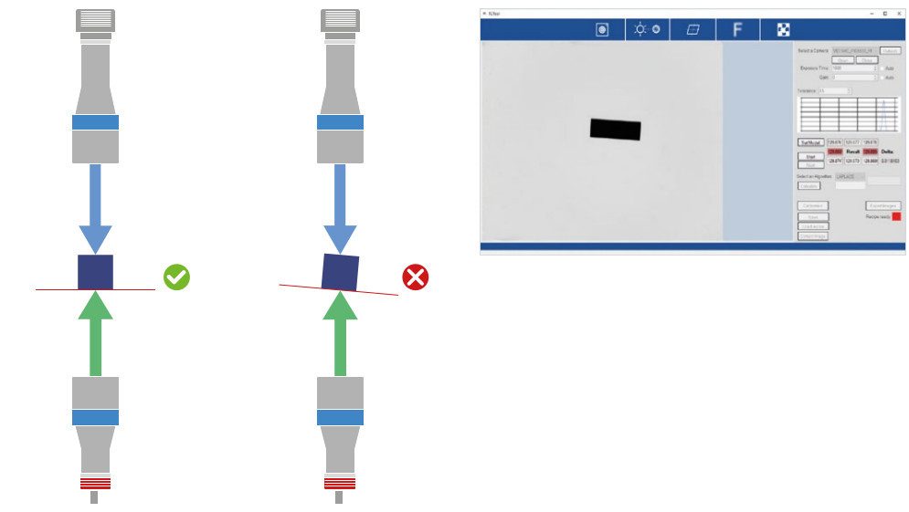
Aligning the object plane
A good alignment of the object plane with the optical axis is essential. Consequences of misalignment are:
• In a backlighting condition we are looking at the object projection, not at its actual profile, hence the image might be affected by some compressions along certain directions.
• Some features might not be at the best focus at the same time, thus compromising the quality of the edge for the measurement.
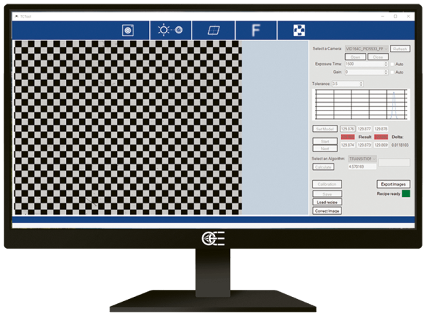
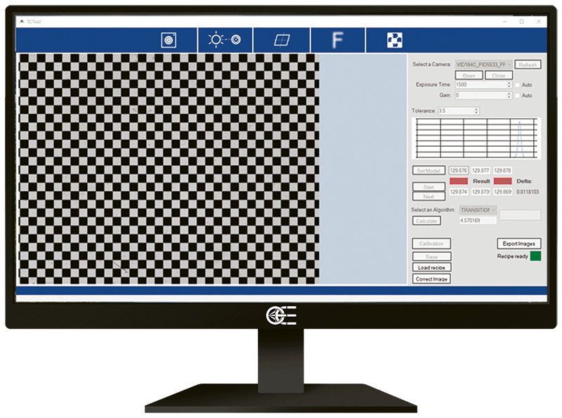
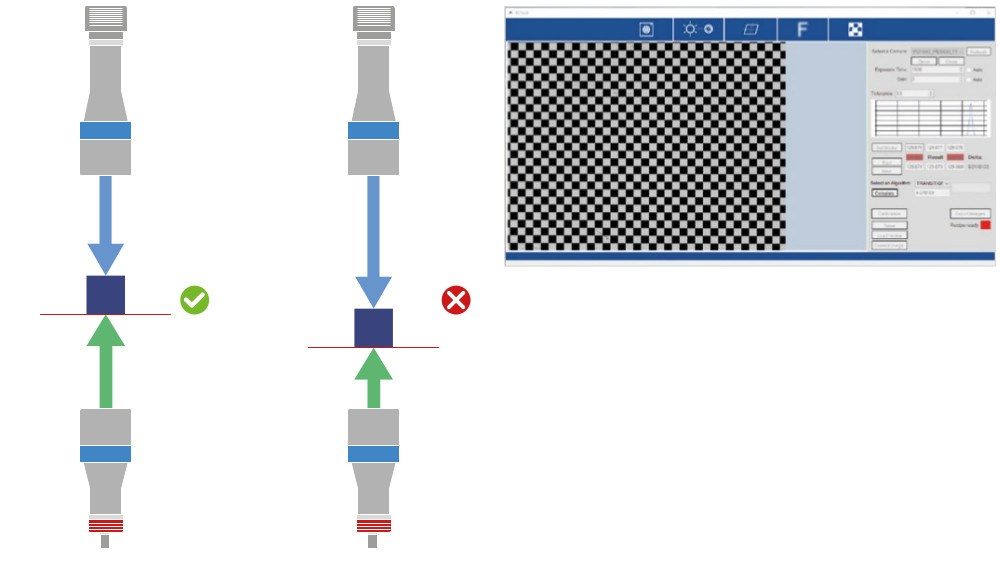
Best focus
This tool gives a numeric index for every image, indicating the proximity to the best focus.
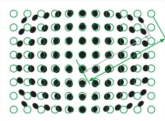
Distortion correction
This tool allows to eliminate the residual optical distortion from telecentric lens – however small, this value must be as close to zero as possible to achieve optimum results. From a single picture of a chessboard pattern covering the whole FoV (such as Opto Engineering® PT series), we get all the information needed to get rid of distortion.
The procedure steps are the following:
- Acquire a single image of the calibration pattern (offline)
- From the picture, a distortion map is created (offline)
- The distortion map is saved on a reference file
- The distortion is eliminated on every new image acquired, recalling the saved distortion map (online)
Step 1. and 2. mean to calibrate the system, hence they are needed just once. Step 4. is repeated on every new image acquired. All these functions are integrated in the library .dll file and in a demo stand-alone software. The demo application can be used for test purpose or to obtain the distortion map, whereas for the actual online correction, the integration of the .dll file is recommended.
Results of an optimized telecentric system
We reviewed the results of using TCLIB Suite to optimize different sets of possible telecentric systems. The results concern the four tools of the Suite as follows:
- lens-light alignment is given in terms of homogeneity of the illumination (standard deviation of the average grey level)
- lens-object plane alignment is given as the lowest value obtained, in degrees
- focus accuracy is given as the sensitivity in mm on the working distance
- distortion calibration is given as repeatability on 20 measurements of a 5 mm gauge block
| TCCP3MHR144-C + LTCLCP144-G + PTCP-S1-HR1-C + ITA120-GM-10C | ||||||||||||||
|---|---|---|---|---|---|---|---|---|---|---|---|---|---|---|
| Field of View | LENS-LIGHT ALIGNMENT as BACKGROUND HOMOGENEITY | OBJECT PLANE ALIGNMENT as BEST (LOWEST) ANGLE BETWEEN PLANES | BEST FOCUS as BEST (LOWEST) UNCERTAINTY ON WD | DISTORTION CALIBRATION as RESULT OF 20 REPEATED MEASUREMENTS | ||||||||||
| 164x120 mm | 4% | 0.012° | +/- 0.5 mm |
| ||||||||||
| TC3MHR144-C + LTCL144-G + PT120-240 (legacy) + ITA120-GM-10C | ||||||||||||||
| Field of View | LENS-LIGHT ALIGNMENT as BACKGROUND HOMOGENEITY | OBJECT PLANE ALIGNMENT as BEST (LOWEST) ANGLE BETWEEN PLANES | BEST FOCUS as BEST (LOWEST) UNCERTAINTY ON WD | DISTORTION CALIBRATION as RESULT OF 20 REPEATED MEASUREMENTS | ||||||||||
| 141x104 mm | 3% | 0.014° | +/- 0.5 mm |
| ||||||||||
| TC3MHR144-C + LTCL144-G + PTCP-S1-HR1-C + ITA120-GM-10C | ||||||||||||||
| Field of View | LENS-LIGHT ALIGNMENT as BACKGROUND HOMOGENEITY | OBJECT PLANE ALIGNMENT as BEST (LOWEST) ANGLE BETWEEN PLANES | BEST FOCUS as BEST (LOWEST) UNCERTAINTY ON WD | DISTORTION CALIBRATION as RESULT OF 20 REPEATED MEASUREMENTS | ||||||||||
| 141x104 mm | 3% | 0.003° | +/- 0.5 mm |
| ||||||||||
| TCCR3M064-C + LTCLCR064-G + PT064-096 + ITA120-GM-10C | ||||||||||||||
| Field of View | LENS-LIGHT ALIGNMENT as BACKGROUND HOMOGENEITY | OBJECT PLANE ALIGNMENT as BEST (LOWEST) ANGLE BETWEEN PLANES | BEST FOCUS as BEST (LOWEST) UNCERTAINTY ON WD | DISTORTION CALIBRATION as RESULT OF 20 REPEATED MEASUREMENTS | ||||||||||
| 62x46 mm | 3% | 0.001° | +/- 0.5 mm |
| ||||||||||
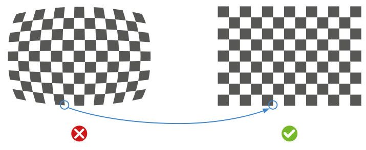
What is distortion calibration?
Every time we use an optical system, i.e. a lens and matching camera, we must face the issue of distortion. The optical distortion of the system can be defined as a bias that causes a set of points to be imaged in different relative positions than the real ones. A typical example is a straight line which is imaged as curved because of the distortion of the lens Fig.1 shows the effect of distortion on a calibration pattern.
The mathematical transformation connecting the original undistorted field of view to the distorted image can be very hard to model, also considering that it can change considerably through the field of view itself.
The first effect of distortion on metrology is the loss of repeatability of the measurements: since an object feature “looks” slightly different depending on where the object is located on the FoV because of distortion, the value of a measurement on that feature will be likely to change every time the object is removed and put back again.
Repeatability of a measurement system
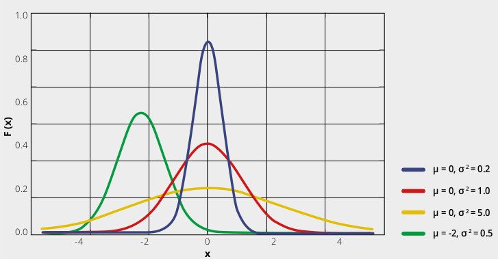
If we measure a through-hole diameter 100 times, the distribution of the results can be approximated by a gaussian curve: results close to the average are very frequent, whereas very different results are unlikely.
The repeatability of the measure is related to the width of the bell: the thinner the width, the harder it will be to find a measure far away from the average. In other words, a certain feature (e.g. a length) will be «almost the same, almost every time». On the other hand, a wide bell represents the situation in which we can’t tell whether a measure is actually different from the expected value (e.g. because it’s a defective part) or it’s a statistically expected outlier given by the low repeatability of our measurement system.
The typical width used is called sigma (or “full width at half
maximum”, FWHM), and it’s directly related to the repeatability. We can
thus establish a direct method to compare the accuracy requirements: if
the tolerance on a measurement is given as multiples of its specific
sigma value, we consequently state the likelihood of an out-of-tolerance
part to present itself. A two sigma compliant object will be within
tolerance 95% of the times. A three sigma object will have a 99.7%
confidence level, rising to 99.99999% at 5 sigma.
Suppose your
distribution has an average value of 150 mm and sigma = 1 mm. The
associated error depends on the confidence value for your application.
In fact, we can state in the feature specs that its length is 150 mm +/-
3 mm, and this will be true 99.7% of the time. On the other hand, if we
want 1 mm to be a 3 sigma tolerance, we must improve our measurement
process until 1 sigma = 0.33 mm.